Property plots

The entries of the Plot menu draw the properties computed by CRYSTAL. The figures are produced by CRYSTALClear and appear in the Plots panel at the bottom of the window, one tab per figure.

Some entries use the output file already open; the others read the data files written by a properties run, and their names end with …. Those files are looked for, and asked for, in the folder of the open output — see working in the calculation’s folder. Plot → Plot font… sets the font of the figures drawn afterwards.

Electronic band structures and densities of states

Plot → Electronic bands & DOS… draws a band structure, a density of states, or the two side by side.

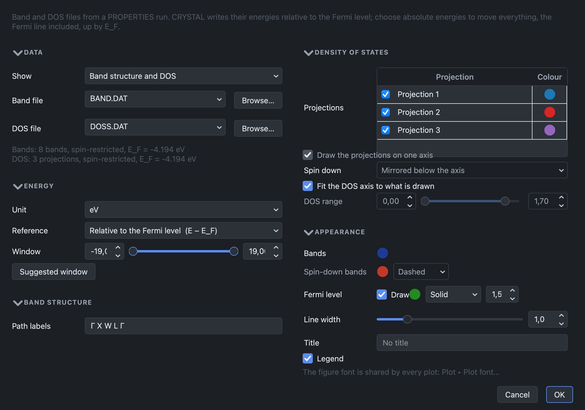
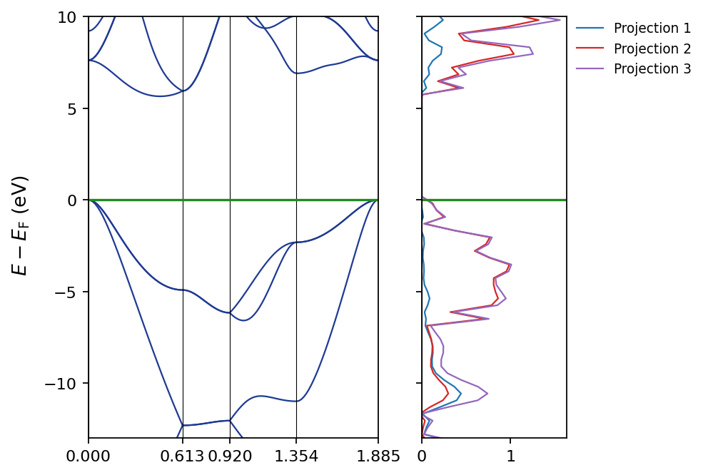
Silicon, along Γ-X-W-L-Γ.

The files. BAND.DAT, DOSS.DAT, *.BAND, *.DOSS, fort.25 and *.f25 are read. Those in the folder of the open output are listed, recognised by their contents rather than by their names, so that a charge-density map or a COOP file is not offered as a band structure. When a folder holds several runs, the band file and the density of states are paired by their Fermi energy, which identifies the SCF they come from; a disagreement is reported.

The energies. CRYSTAL writes them relative to the Fermi level. They can be plotted that way or as absolute energies, in which case the Fermi energy is added back and the line marking it moves with the data. Units are eV or Hartree. The window is taken from the contents of the file — from the first wide gap below the Fermi level, which separates the valence bands from the core levels, to as far above — and Suggested window restores it.

The rest. The projections of the density of states, with their names and colours; the treatment of the spin-down component; the labels of the path; and the colours, styles and widths of the lines.

Vibrational spectra

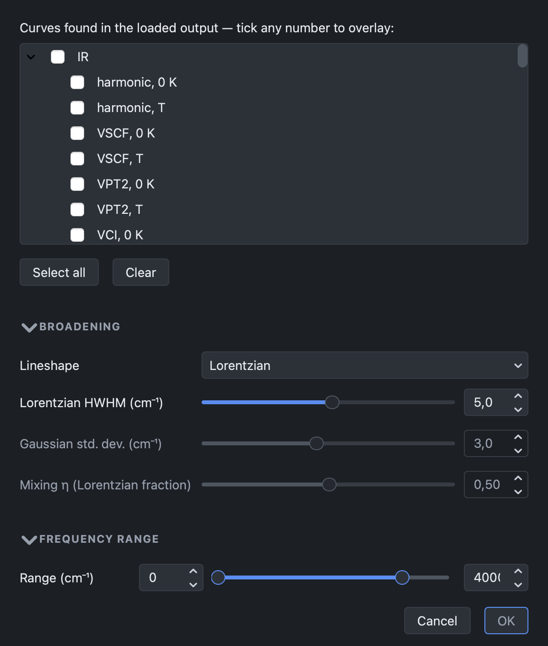
Plot → Vibrational spectra… lists the curves contained in the output: infrared, Raman with its polarisations, and their anharmonic (VSCF, VCI) counterparts where present.

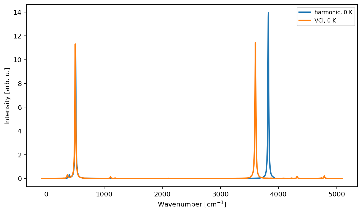
Brucite: the harmonic spectrum and its VCI counterpart, which shows the anharmonic shift.

Several curves may be selected at once, which is the usual case: the single-crystal Raman components on the same axes show the anisotropy, and a harmonic curve under its anharmonic counterpart shows the shift. The broadening is chosen in the same dialog — pseudo-Voigt, Lorentzian, Gaussian or a stick spectrum — and only the widths used by the chosen lineshape are enabled.

Anharmonic calculations

• VCI states… — the states of a VCI calculation, as a heatmap or a Sankey diagram.

• Anharmonic scan… — the scanned potential.

• Anharmonic PES… — one- and two-dimensional cuts of the potential energy surface, with the wavefunctions and probability densities of a double well.

Properties read from the output

These entries use the open output file and are enabled when it contains the data they need.

• Elastic properties — Young’s modulus, linear compressibility, shear modulus and Poisson’s ratio, as three-dimensional surfaces and as sections through them.

• Equation of state.

• Phonon band structures and densities of states, from the data files of a dispersion calculation.

• Simulated XRD patterns.

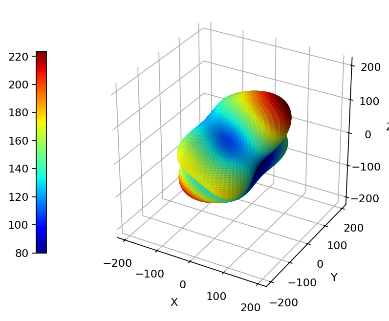
The directional Young’s modulus of coesite.

Crystalline orbitals

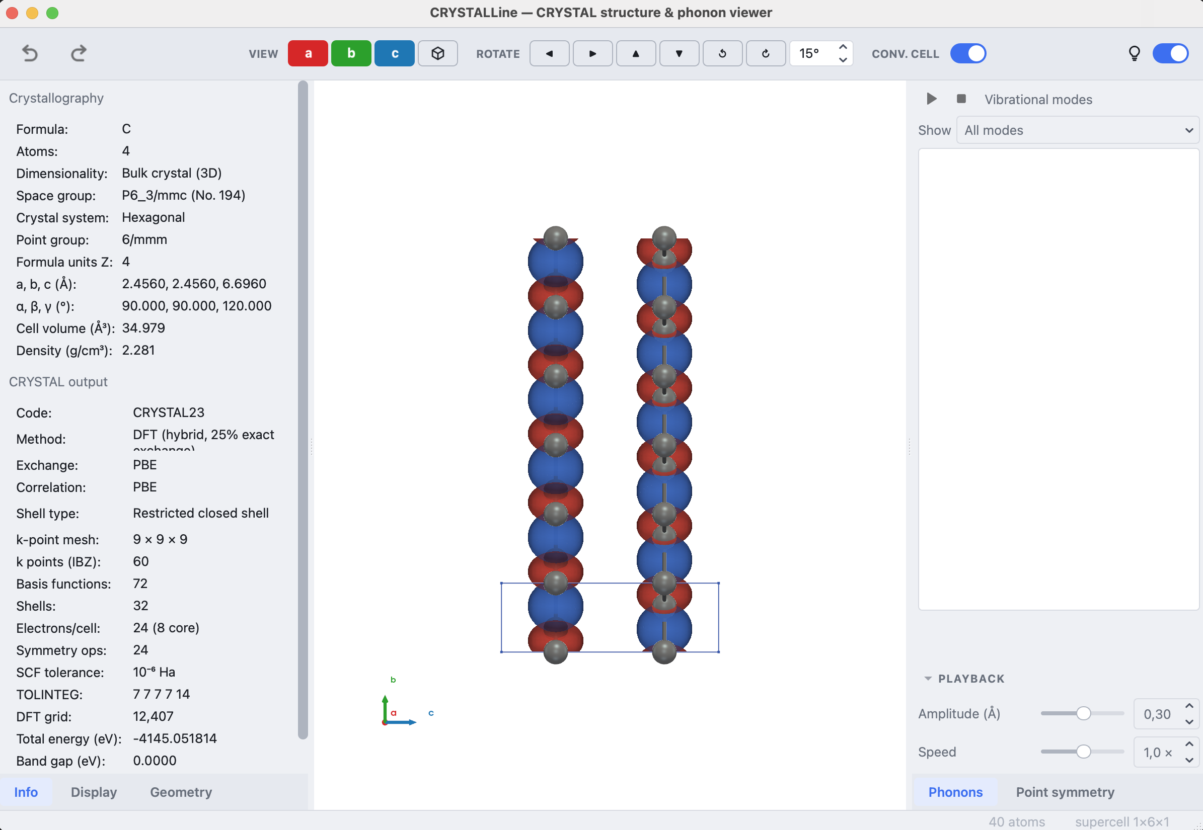
Plot → Crystalline orbitals… reads the files written by the ORBITALS keyword and draws the orbital in the 3D view rather than in the plot panel; Clear orbital removes it.

Electron density and electrostatic potential

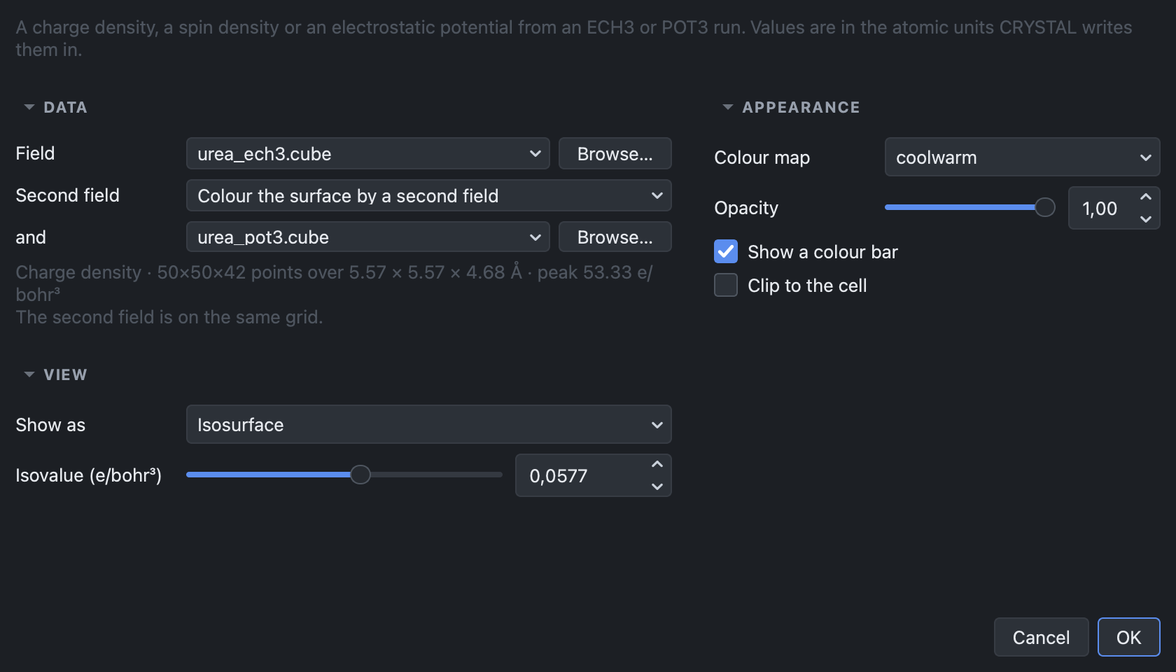
Plot → Electron density & potential… draws the grids written by ECH3 and POT3 over the structure, in the 3D view; Clear field removes them.

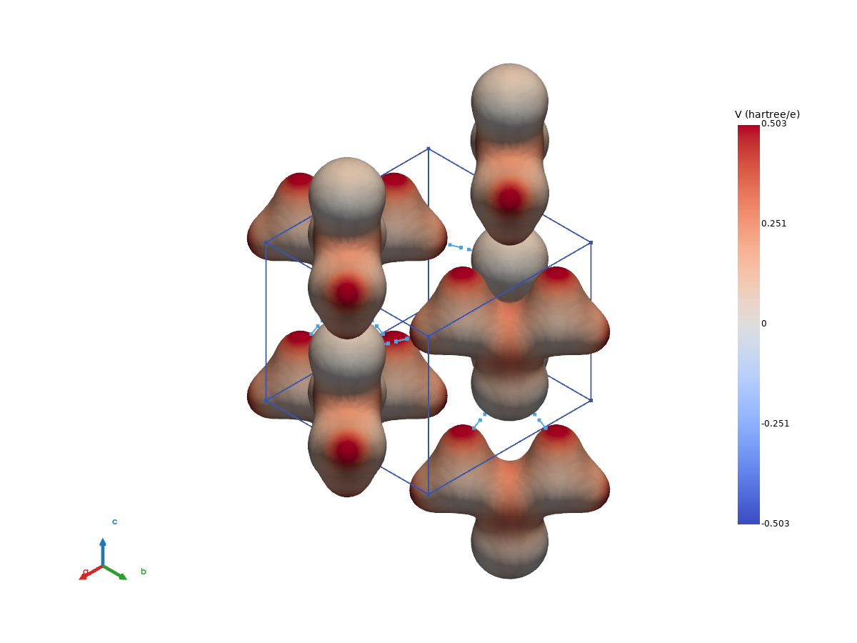
Urea: the charge density at 0.058 e/bohr³, coloured by the electrostatic potential.

The CUBE files and fort.31 are found in the folder of the open output and recognised by their content, with the grids of the open structure offered first. A field is drawn either as an isosurface, which opens at a level that clears the drawn atoms, or on a lattice plane given by its Miller indices in the conventional cell; the crystal in front of the plane is cut away and the atoms lying in it are marked. A colour bar can be added. A second field either colours the surface — the potential on the density, as above — or is subtracted from the first.