Simulating Vibrational Spectra

In this notebook, we’ll use CRYSTALClear to turn raw vibrational data from CRYSTAL simulations into clear, easy-to-read spectra — no tedious manual parsing required.

Infrared Spectrum

CRYSTALClear comes with a handy plotting function called plot_cry_spec (in the plot module).

It’s designed to take vibrational data you’ve already extracted from a CRYSTAL output and turn it into a polished spectrum — in just one line.

Here’s the basic idea:

1. Load your CRYSTAL output into a Crystal_output object.

2. Extract IR data by running the .get_IR method on that object. This step create the .IR_HO_0K attribute containing harmonic frequencies and IR intensities (numpy 2D array).

3. Plot the IR spectrum by passing this attribute to plot_cry_spec.

Let’s create a Crystal_output object (CO):

from CRYSTALClear.crystal_io import Crystal_output
CO = Crystal_output("thiourea_pbed3_Ahlrichs-pVTZ_freqcalc.out")

Then, we can extract IR data with this one-liner:

CO.get_IR()

<CRYSTALClear.crystal_io.Crystal_output at 0x107b7ffd0>

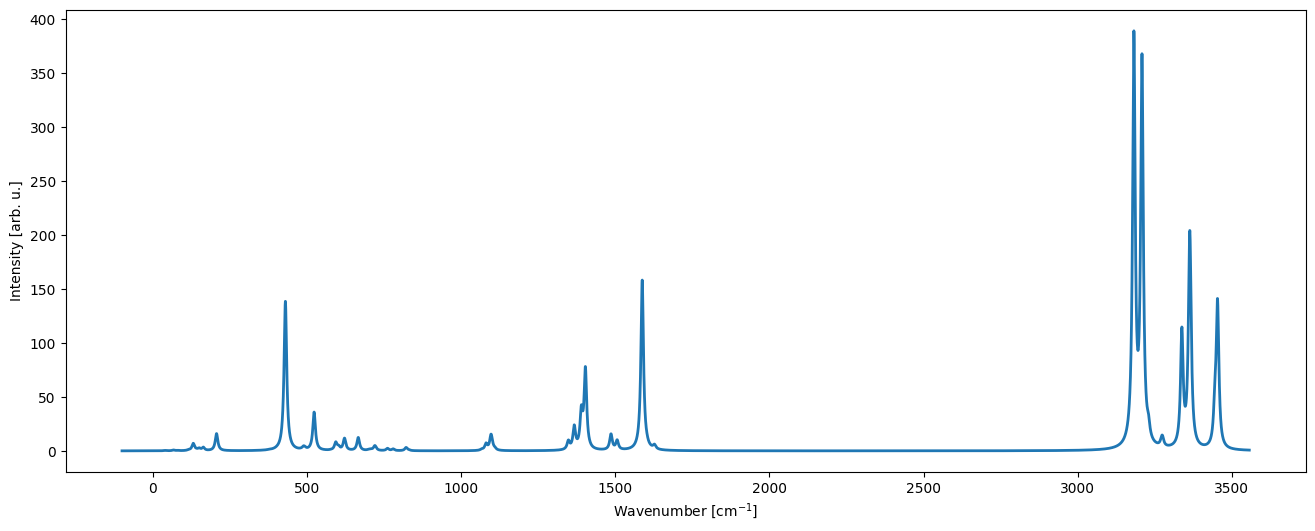
We can finally create a plot by making use of the plot_cry_spec function:

import CRYSTALClear.plot as CCplt
CCplt.plot_cry_spec(CO.IR_HO_0K)

(<Figure size 1600x600 with 1 Axes>,
 <AxesSubplot: xlabel='Wavenumber [cm$^{-1}$]', ylabel='Intensity [arb. u.]'>)

plot_cry_spec supports several optional arguments that allow you to control how the spectrum is displayed.

A key argument is typeS, which defines the line shape:

• "bars" → Dirac delta lines (stick spectrum)

• "lorentz" → Lorentzian peaks (default)

• "gauss" → Gaussian peaks

• "pvoigt" → Pseudo-Voigt peaks (mixture of Lorentzian and Gaussian)

When you choose a peak shape with typeS, a few additional parameters control exactly how the peaks are drawn:

• bwidth → Half-width at half-maximum (HWHM) for a Lorentzian profile.

  • Larger bwidth → broader peaks with slower decay in the tails.

  • Smaller bwidth → sharper, narrower peaks.

• stdev → Standard deviation for a Gaussian profile.

  • Larger stdev → wider, more “blurred” peaks.

  • Smaller stdev → peaks become sharper and more defined.

• eta → Fraction of Lorentzian character in a pseudo-Voigt profile.

  • eta = 0 → pure Gaussian

  • eta = 1 → pure Lorentzian

  • Values in between blend the two shapes for a balanced peak form.

Other optional arguments include style, labels, line width, frequency range, etc. For a full list of arguments, you can have a look at the documentation. Since the function returns fig and ax, you can still use all Matplotlib features to further customize the plot.

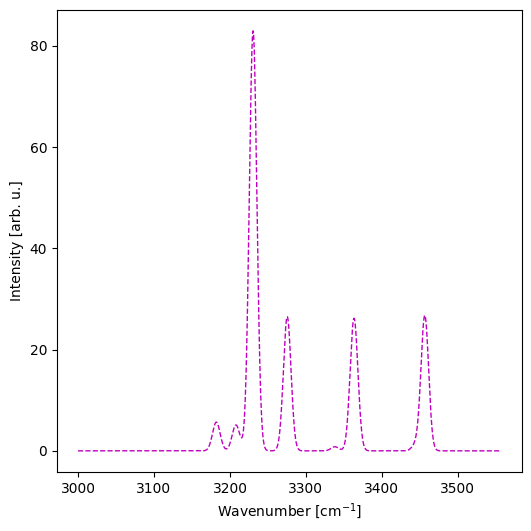
Raman Spectrum

The process is analogous to IR. After computing Raman intensities, pass the result to plot_cry_spec.

CO.get_Raman()
CCplt.plot_cry_spec(CO.Ram_HO_0K_tot, typeS="gauss", stdev=5, fmin=3000, style="m--", figsize=[6,6], linewidth=1)

(<Figure size 600x600 with 1 Axes>,
 <AxesSubplot: xlabel='Wavenumber [cm$^{-1}$]', ylabel='Intensity [arb. u.]'>)

Combined Spectra

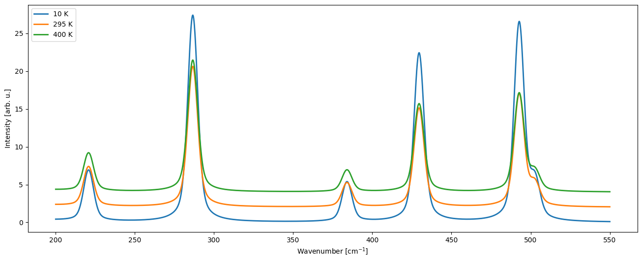
Sometimes you want to see how the spectrum changes under different conditions — for example, the Raman spectrum of a compound at various temperatures or using different laser wavelengths.

The plot_cry_spec_multi function is perfect for this. It accepts a list of spectra and plots them on the same axes. Optional arguments like style and label now require lists of the same length as the number of spectra. Each list entry corresponds to a spectrum in the same order.

# Raman spectra of the same material (alpha quartz) at three temperatures
qua10K = Crystal_output('qua_hf_2d_f-raman_10K_550nm.out')
qua295K = Crystal_output('qua_hf_2d_f-raman_295K_488nm.out')
qua400K = Crystal_output('qua_hf_2d_f-raman_400K_550nm.out')

qua10K.get_Raman()
qua295K.get_Raman()
qua400K.get_Raman()

<CRYSTALClear.crystal_io.Crystal_output at 0x117f04c10>

Let’s plot these spectra all together!

CCplt.plot_cry_spec_multi([qua10K.Ram_HO_0K_tot, qua295K.Ram_HO_0K_tot, qua400K.Ram_HO_0K_tot], typeS="pvoigt", label=['10 K', '295 K', '400 K'], fmin=200, fmax=550,  offset=2)

(<Figure size 1600x600 with 1 Axes>,
 <AxesSubplot: xlabel='Wavenumber [cm$^{-1}$]', ylabel='Intensity [arb. u.]'>)