Transport properties plot#
CRYSTALClear contains functions to read the computed Seebeck Coefficient (\(S\)) and Electrical Conductivity (\(\sigma\)) from a PROPERTIES calculation and to compute and plot the thermoelectrical Power Factor \((PF=S^2*\sigma)\) and the Figure of Merit (\(ZT=(PF*T)/K_{tot}\), where \(K_{tot}\) is the total thermal conductivity). Please, note that the first essential step consists in running a properties calculation with CRYSTAL by using the keyword BOLTZTRA (see the User’s Manual for details). Below, we will show how to exploit such functionalities referring to calculations on the ZrNiSn Half Heusler alloy.
[4]:
from CRYSTALClear.crystal_io import *
import CRYSTALClear.plot as CCplt
At first we will create two seebeck objects, seebeck and seebeck1, reading two SEEBECK.DAT files.
[2]:
seebeck = Properties_output().read_cry_seebeck('transport_zrnisn_SEEBECK.DAT')
[16]:
seebeck1 = Properties_output().read_cry_seebeck('transport_zrnisn_antisito_SEEBECK.DAT')
We can plot them as a function of the chemical potential or of the charge carrier concentration, using the plot_cry_seebeck_potential and the plot_cry_seebeck_carrier funcitons. To acquire information on the structure of the function we can write ?function name and run the cell. The plotting functions generate matplotlib figure objects.
[9]:
?CCplt.plot_cry_seebeck_potential
Signature: CCplt.plot_cry_seebeck_potential(seebeck_obj, direction, temperature)
Docstring:
Plot the Seebeck coefficient as a function of chemical potential.

Args:
    seebeck_obj (object): Seebeck object containing the data for the Seebeck coefficient.
    direction (str): choose the direction to plot among 'S_xx', 'S_xy', 'S_xz', 'S_yx', 'S_yy', 'S_yz', 'S_yz', 'S_zx', 'S_zy', 'S_zz'.
    temperature (value/str): choose the temperature to be considered or 'all' to consider them all together

Returns:
    Figure object

Notes:
    - Plots the Seebeck coefficient as a function of chemical potential for each temperature.
    - Distinguishes between n-type and p-type conduction with dashed and solid lines, respectively.
File:      c:\users\ascri\onedrive\desktop\dottorato_secondo_anno\tutorial_2022\electron_transport_properties\plot.py
Type:      function
[5]:
plot_seebeck = CCplt.plot_cry_seebeck_carrier(seebeck,'s_xx','all')
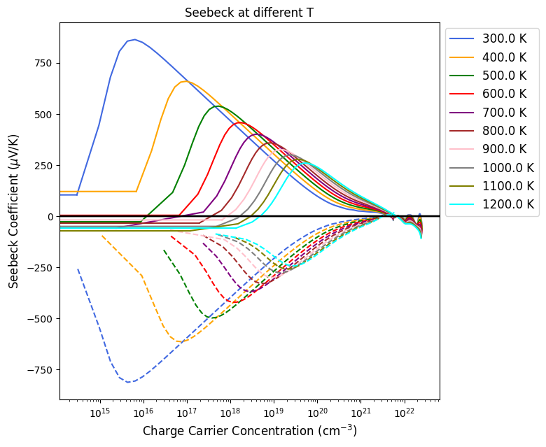
To differentiate transport coefficients due to n-type or p-type conduction (electrons or holes as majority carriers) dashed and solid lines are used, respectively.
<Figure size 640x480 with 0 Axes>
[ ]:
plot_seebeck.savefig('seebeck_potential',dpi=300)
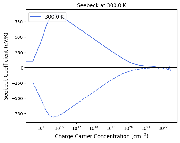
Plot seebeck versus the charge carrier concentration
[9]:
CCplt.plot_cry_seebeck_carrier(seebeck,'s_xx',300)
To differentiate transport coefficients due to n-type or p-type conduction (electrons or holes as majority carriers) dashed and solid lines are used, respectively.
[9]:
<Figure size 640x480 with 0 Axes>
<Figure size 640x480 with 0 Axes>
Now we will create two sigma objects, sigma and sigma1, reading two SIGMA.DAT files.
[11]:
sigma = Properties_output().read_cry_sigma('transport_zrnisn_SIGMA.DAT')
[12]:
sigma1 = Properties_output().read_cry_sigma('transport_zrnisn_antisito_SIGMA.DAT')
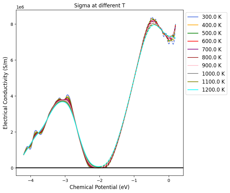
We can plot the electrical conductivity as a function of the chemical potential or of the charge carrier concentration, using the plot_cry_sigma_potential or plot_cry_sigma_carrier functions.
[13]:
CCplt.plot_cry_sigma_potential(sigma,'s_xx','all')
To differentiate transport coefficients due to n-type or p-type conduction (electrons or holes as majority carriers) dashed and solid lines are used, respectively.
[13]:
<Figure size 640x480 with 0 Axes>
<Figure size 640x480 with 0 Axes>
If we want to compare on the same plot Seebeck coefficients or electrical conductivities coming from different file, we can use the plot_cry_multiseebeck and plot_cry_multisigma functions.
[14]:
?CCplt.plot_cry_multiseebeck
Signature:
CCplt.plot_cry_multiseebeck(
    direction,
    temperature,
    minpot,
    maxpot,
    *seebeck,
)
Docstring:
Plot the seebeck coefficient from different files.

Args:
    direction (str): choose the direction to plot among 'S_xx', 'S_xy', 'S_xz', 'S_yx', 'S_yy', 'S_yz', 'S_yz', 'S_zx', 'S_zy', 'S_zz'.
    temperature (value): choose the temperature to be considered
    minpot (value): lower value of chemical potential you want to plot in eV
    maxpot (value): higher value of chemical potential you want to plot in eV
    *seebeck (obj): Variable number of seebeck objects containing the data for the Seebeck coefficient.

Returns:
    Figure object

Notes:

    - Plots the seebeck coefficient for each seebeck object.
    - Differentiates transport coefficients due to n-type or p-type conduction using dashed and solid lines.
File:      c:\users\ascri\onedrive\desktop\dottorato_secondo_anno\tutorial_2022\electron_transport_properties\plot.py
Type:      function
[17]:
CCplt.plot_cry_multiseebeck('s_xx',300,-6,-1,seebeck, seebeck1,)
To differentiate transport coefficients due to n-type or p-type conduction (electrons or holes as majority carriers) dashed and solid lines are used, respectively.
[17]:
<Figure size 640x480 with 0 Axes>
<Figure size 640x480 with 0 Axes>
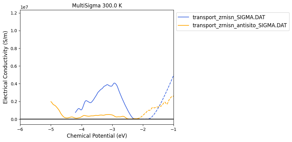
Plot multisigma
[17]:
CCplt.plot_cry_multisigma('s_xx',300,-6,-1,sigma, sigma1)
To differentiate transport coefficients due to n-type or p-type conduction (electrons or holes as majority carriers) dashed and solid lines are used, respectively.
[17]:
<Figure size 640x480 with 0 Axes>
<Figure size 640x480 with 0 Axes>
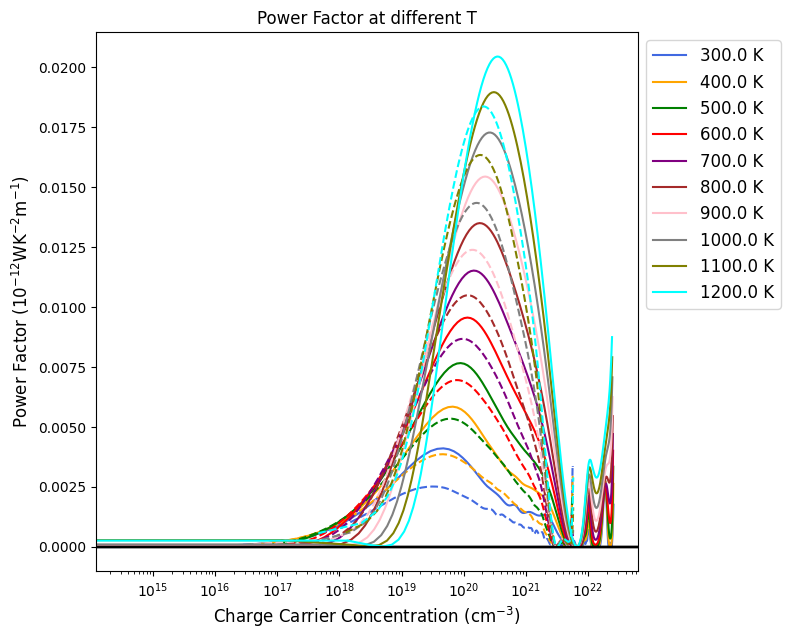
To compute and plot the Power Factor and ZT we can use the plot_cry_powerfactor and plot_cry_zt functions.
[18]:
CCplt.plot_cry_powerfactor_carrier(seebeck, sigma,'pf_xx','all')
To differentiate transport coefficients due to n-type or p-type conduction (electrons or holes as majority carriers) dashed and solid lines are used, respectively.

[18]:
<function matplotlib.pyplot.gcf() -> 'Figure'>
[21]:
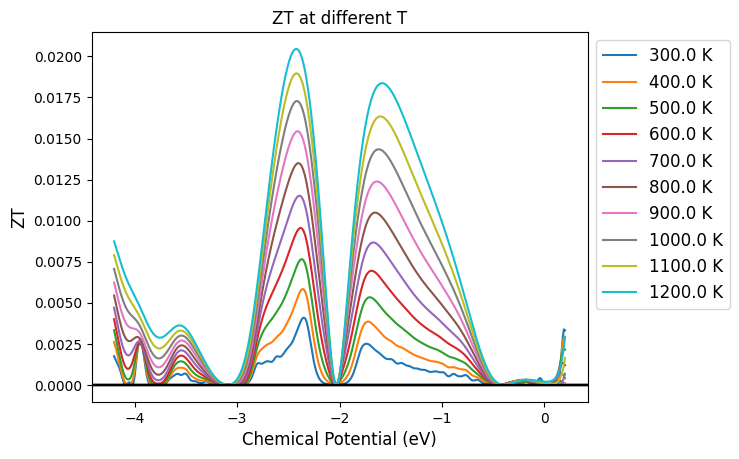
?CCplt.plot_cry_zt
Signature: CCplt.plot_cry_zt(seebeck_obj, sigma_obj, direction, temperature, ktot)
Docstring:
Plot the ZT value for different temperatures.

Args:
    seebeck_obj (obj): Seebeck object containing the data for the Seebeck coefficient.
    sigma_obj (obj): Sigma object containing the data for the electrical conductivity.
    direction (str): choose the direction to plot among 'ZT_xx', 'ZT_xy', 'ZT_xz', 'ZT_yx', 'ZT_yy', 'ZT_yz', 'ZT_yz', 'ZT_zx', 'ZT_zy', 'ZT_zz'.
    temperature (value/str): choose the temperature to be considered or 'all' to consider them all together
    ktot (value): alue of the total thermal conductivity (ktot) in W-1K-1m-1

Returns:
    Figure object

Notes:
    - Calculates the ZT value using the Seebeck coefficient and electrical conductivity data.
    - Plots the ZT value for each temperature as a function of the chemical potential.
File:      c:\users\ascri\onedrive\desktop\dottorato_secondo_anno\tutorial_2022\electron_transport_properties\plot.py
Type:      function
[20]:
CCplt.plot_cry_zt(seebeck,sigma,'zt_xx','all',10)
[20]:
<function matplotlib.pyplot.gcf() -> 'Figure'>
[ ]: